Molecular Weight Models

The are many models for estimating SCN component molecular weights. In this section, some of the most common models are covered.

Table Values - Katz-Firoozabadi & Whitson

The first type, and most likely the most commonly used although it is not recommended is to use a fixed set of table values like those given by Katz and Firoozabadi or Whitson shown in Table 1 and Figure 1. These are so common because they are typically used in laboratory PVT reports when reporting the sample molar compositions. The measured compositions (at least for C₅₊) are almost exclusively measured using a flaming ionizing detector (FID) which correlated its measured properties with the mass amount. This means that when laboratories give mole compositions up to for example C₃₀₊ like in the Duvernay data, they are using some default set of molecular weights that are most likely taken from the Katz-Firoozabadi or Whitson tables.

Table 1: Katz-Firoozabadi and Whitson SCN component molecular weights for C₆₊. katz_firoozabadi_table

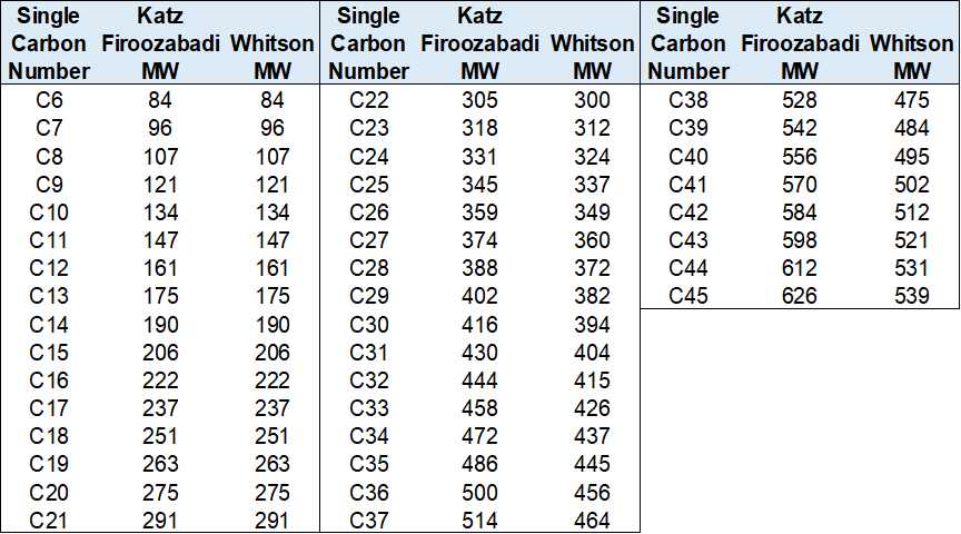
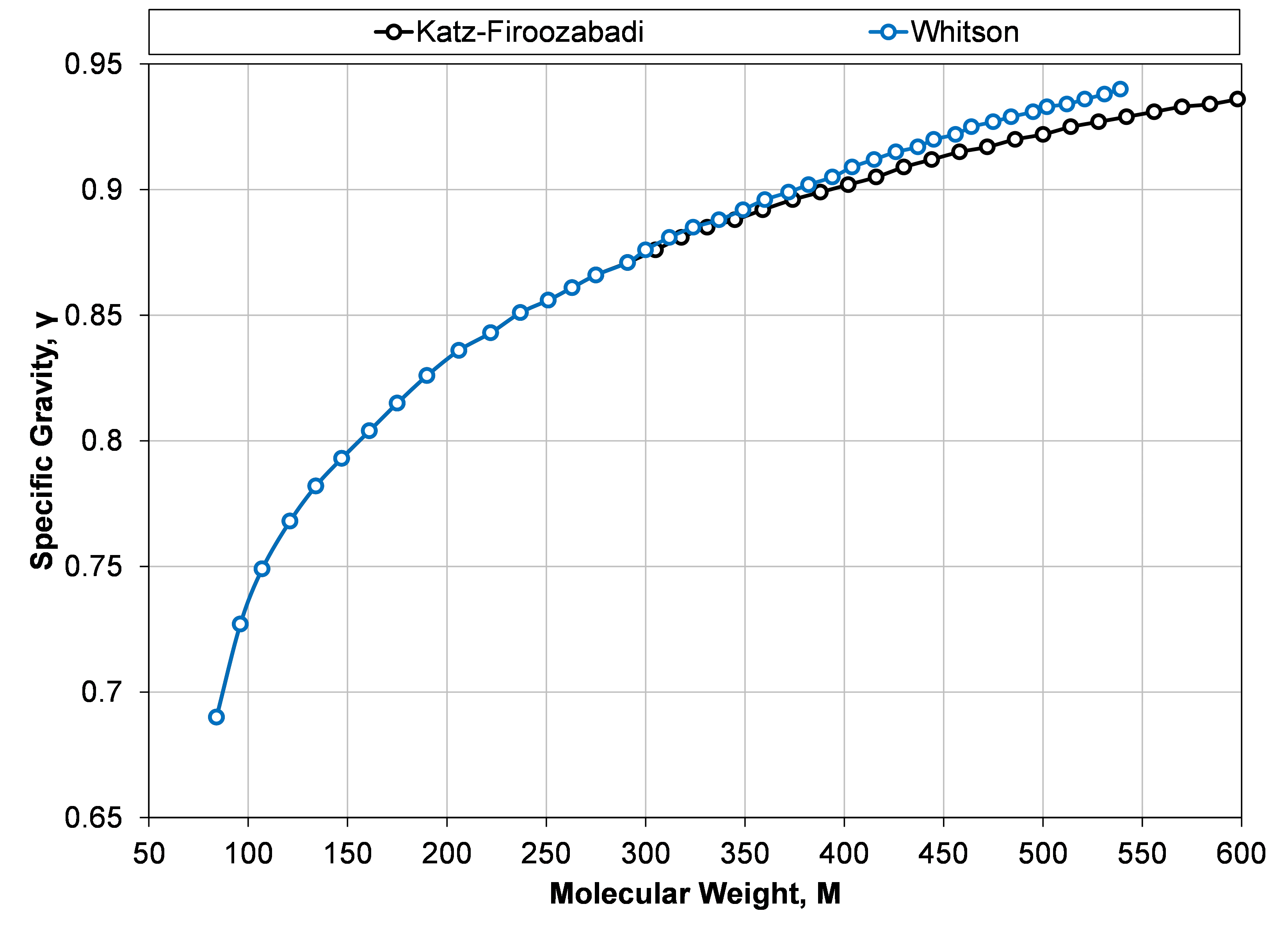katz_firoozabadi_plot Figure 1: Specific gravity and molecular weight for SCN components from C₆ to C₄₅ taken from the Katz-Firoozabadi and Whitson tables.

Normal Paraffin Model

The upper bound for the SCN component molecular weights are the normal paraffin molecular weights. The equation for these molecular weights is well known and is derived in Figure 2 below.

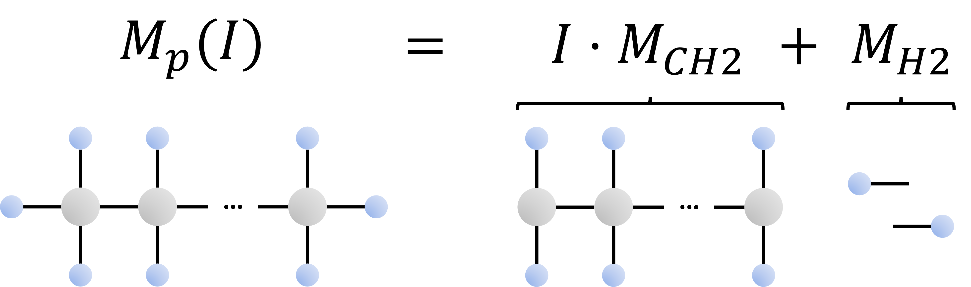normal_paraffin_figure Figure 2: Visual proof of how to calculate the normal paraffin molecular weight. Grey circles are carbon atoms and the blue circles are hydrogen atoms.

The normal paraffin molecular weight ($M_p (I)$) is given by

$\begin{equation}\label{eq:normal_paraffin_mw_correlation} M_p(I) = M_{CH2} I + M_{H2} \end{equation}$ $\begin{equation}\label{eq:CH2_and_H2_mw} M_{CH2}=14.0269, M_{H2}=2.01588 \end{equation}$

where I is the paraffin carbon number (e.g. for n-C₇ then I = 7). The values given in Equation \eqref{eq:CH2_and_H2_mw} are the molecular weight of a carbon and two hydrocarbon atoms ($M_{CH2}$), and the molecular weight of two hydrocarbon atoms ($M_{H2}$) respectively. From the normal paraffin molecular weight ($M_p (I)$) it is possible to estimate the normal paraffin normal boiling point ($T_b (I)$) from

$\begin{equation}\label{eq:tb_twu_correlation} T_b(I)=\exp⁡(5.71419+2.71579 θ-0.28659 θ^2-39.8544 θ^{-1}-0.122488 θ^{-2})-24.7522 θ+35.3155 θ^2 \end{equation}$ $\begin{equation}\label{eq:theata_definition} θ=\ln⁡[M_p (I)] \end{equation}$

From the normal paraffin normal boiling point ($T_b (I)$) it is possible to estimate the normal paraffin critical temperature ($T_{cp} (I)$) using

$\begin{equation}\label{eq:paraffin_tc} T_{cp}(I)=T_b [0.533272+1.91017⋅10^{-4} T_b+7.79681⋅10^{-8} T_b^2-2.84376⋅10^{-11} T_b^3+\frac{9.59468⋅10}{(0.01 T_b)^{13}} ]^{-1} \end{equation}$

and the normal paraffin specific gravity ($\gamma_p$) is given by

$\begin{equation}\label{eq:paraffin_sg} \gamma_p=0.843593-0.12864 α-3.36159 α^3-13749.5 α^{12} \end{equation}$ $\begin{equation}\label{eq:alpha_definition} \alpha=1-\frac{T_b}{T_{cp}} \end{equation}$

where $T_b$ in Equations \eqref{eq:paraffin_tc}, \eqref{eq:paraffin_sg}, and \eqref{eq:alpha_definition} refers to the normal paraffin normal boiling point ($T_b (I)$) as defined in Equation \eqref{eq:tb_twu_correlation}.

Generalized Paraffin Model and the Pedersen Model

There is no naturally occurring hydrocarbon system that only consists of normal paraffins, and the SCN component molecular weights will therefore not be described accurately by Equation \eqref{eq:normal_paraffin_mw_correlation}. A modification to this model is to generalize Equation \eqref{eq:normal_paraffin_mw_correlation} to be

$\begin{equation}\label{eq:generalized_paraffin_mw_correlation} M_p(I) = M_{CH2} I + M_{H2} \end{equation}$

where $M_{CH2}$ is given in \eqref{eq:CH2_and_H2_mw} and h is some value bounded by

$\begin{equation}\label{eq:h_constraint} h≤M_{H2} \end{equation}$

which will be referred to as the generalized paraffin model.

If $h=M_{H2}$ then Equation \eqref{eq:generalized_paraffin_mw_correlation} is the same as Equation \eqref{eq:normal_paraffin_mw_correlation}. It is not a requirement, but h is sometimes bounded on the lower end such that $M_{CH2}(I-1)<h$ to keep the SCN molecular weight above the normal paraffin molecular weight of the previous carbon number. This is not always the case, as fluids with a large number of aromatic components can have molecular weights well into the previous carbon number’s normal paraffin molecular weight. A specific example is benzene, which is in SCN C₇, but has a molecular weight of 78.11 which is less than normal hexane’s (n-C₆) molecular weight of 86.178.

The Pedersen model assumes a constant value of h equal to -4 such that

$\begin{equation}\label{eq:pedersen_mws} M(I)=M_{CH2} I-4 \end{equation}$

where $M_{CH2}$ is defined in Equation \eqref{eq:CH2_and_H2_mw}.

Effective Paraffin Model

The goal of this section is to utilize the specific gravity model to estimate representative molecular weights. Given a gravity model ($\gamma(M)$) that yields a specific gravity for a given molecular weight, that has been characterized to flashed oil data, then it is possible to estimate an effective paraffin molecular weight.

First, let’s define the effective carbon number $(i)$ as a number between a given paraffin carbon number $(I)$ and the previous paraffin carbon number $(I-1)$. The formal definition is given by

$\begin{equation}\label{eq:effective_carbon_number_constraint} I-1<i≤I \end{equation}$

The relationship between the effective carbon number, the paraffin molecular weight ($M_p(I)$) and the effective paraffin molecular weight ($M_p(i)$) is given by

$\begin{equation}\label{eq:effective_paraffin_model} M_p(i)=M_p (I)-δ⋅M_{CH2} \end{equation}$ $\begin{equation}\label{eq:delta_constraint} 0<δ≤1 \end{equation}$

In the limits of $\delta$ the effective paraffin molecular weight ($M_p(i)$) equals the actual normal paraffin molecular weight ($M_p(I)$) when $\delta=0$, and tends to the normal paraffin molecular of the previous carbon number ($M_p(I-1)$) as $\delta \to 1$. The deviation parameter ($\delta$) is similar to the Jacoby characterization factor ($J_a$) in the sense that it represents the degree of paraffinicity or aromaticity as $\delta=0$ or $\delta \to 1$ respectively.

The formulation between the effective carbon number in Equation \eqref{eq:effective_carbon_number_constraint} and the generalized normal paraffin model given in Equation \eqref{eq:generalized_paraffin_mw_correlation} is given by $h=M_{H2}-\delta \cdot M_{CH2}$.

In this section, the goal is to find an explicit expression for the deviation parameter ($\delta$) and finalize the workflow for estimating the molecular weights ($M$) of a single carbon number component based only on the carbon number ($I$) and the specific gravity model ($\gamma(M)$).

Because the deviation parameter (δ) has similarities to the Jacoby characterization factor ($J_a$) given in Section 1, the Jacoby gravity model will be the starting point and will be used as a basis for defining the deviation factor. The metric that determines the degree of aromaticity is chosen to be the difference between the gravity model result at the normal paraffin molecular weight ($\gamma[M_p(I)]$) and the normal paraffin gravity ($\gamma_p$). This relationship is given by

$\begin{equation}\label{eq:delta_sg_metric} Δγ(I)=γ[M_p(I)]-γ_p \end{equation}$

Using the Jacoby gravity model to estimate the gravities in Equation \eqref{eq:delta_sg_metric} yields

$\begin{equation}\label{eq:delta_sg_metric_with_jacoby} Δγ(I)=0.8468-\frac{15.8}{M_p} +J_a (0.2456-\frac{1.77}{M_p})-(0.8468-\frac{15.8}{M_p}) \end{equation}$

The Jacoby characterization factor for the normal paraffin specific gravity ($\gamma_p$) is, by definition, zero. Simplifying Equation \eqref{eq:delta_sg_metric_with_jacoby} yields

$\begin{equation}\label{eq:delta_sg_metric_with_jacoby_simplified} Δγ(I)=J_a (0.2456-\frac{1.77}{M_p}) \end{equation}$

where the Jacoby characterization factor can go from zero to some upper value that encloses most aromatic components as shown in Figure 3. Setting an upper bound for the Jacoby factor ($J_a^*$), it is possible to normalize Equation \eqref{eq:delta_sg_metric_with_jacoby_simplified} to go from 0 to 1 as follows

$\begin{equation}\label{eq:delta_definition_with_jacoby} δ=\frac{Δγ(I)}{J_a^* (0.2456-\frac{1.77}{M_p})}=\frac{γ[M_p (I)]-γ_p}{J_a^* (0.2456-\frac{1.77}{M_p})} \end{equation}$

The relationship given in Equation \eqref{eq:delta_definition_with_jacoby} will be the choice of deviation parameter in this article. The only remaining unknown is the value of the upper limit Jacoby characterization factor ($J_a^*$). 3 shows the Jacoby specific gravity – molecular weight relationship for $J_a=1$, $J_a=1.25$, $J_a=1/0.7$ and $J_a=1.5$, together with a variety of hydrocarbon components (for C₅₊).

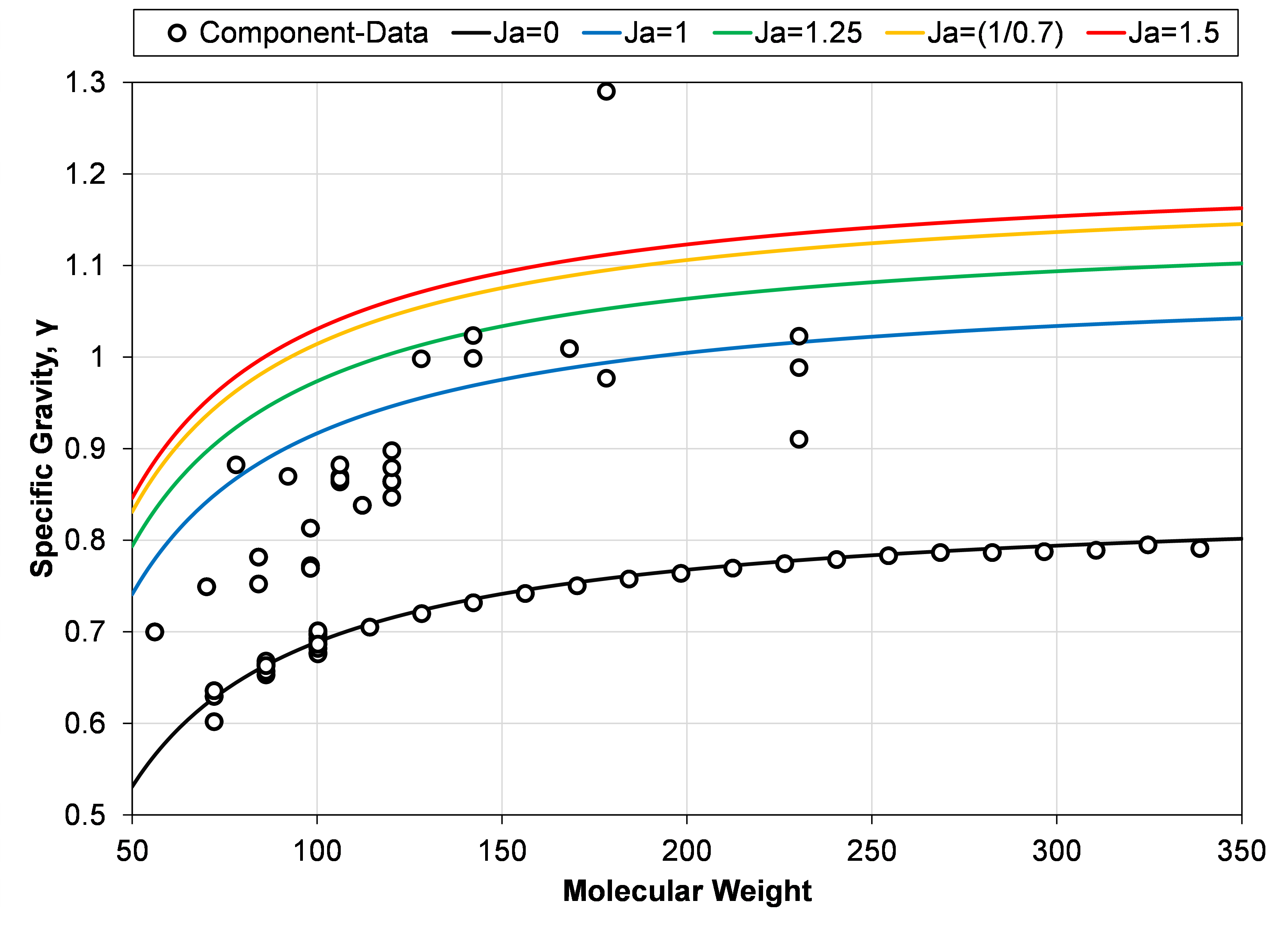paraffin_aromatic_bound Figure 3: Specific gravity and molecular weights for hydrocarbon components (C₅₊) as symbols, and Jacoby specific gravity relationship for Jacoby factors ranging from 0 to 1.5.

Based on the results shown in Figure 3, an empirical choice of the upper limit Jacoby factor ($ J_a^{*} $) can be chosen between 1.25 and 1.5. An arbitrary choice was made in this article to set the upper limit to $J_a^{*}=1/0.7$, such that Equation \eqref{eq:delta_definition_with_jacoby} simplifies to

$\begin{equation}\label{eq:delta_definition_with_jacoby_with_specific_Ja} δ=0.7 \frac{γ[M_p (I)]-γ_p}{(0.2456-1.77/M_p)} \end{equation}$

The equation for the effective carbon number can be derived by combining Equations \eqref{eq:normal_paraffin_mw_correlation}, \eqref{eq:effective_paraffin_model}, and \eqref{eq:delta_definition_with_jacoby_with_specific_Ja}

$\begin{equation}\label{eq:simplified_ep_model_part_1} M_p (i)=M_p (I)-δ⋅M_{CH2}=(M_{CH2} I+M_{H2} )-δ⋅M_{CH2} \end{equation}$ $\begin{equation}\label{eq:simplified_ep_model} M_p (i)=[M_{CH2} (I-δ)]+M_{H2}=M_{CH2}⋅i+M_{H2} \end{equation}$ $\begin{equation}\label{eq:effective_carbon_number_definition} i=I-\delta \end{equation}$

With this choice of deviation parameter, the single carbon number component properties can be within the blue region shown in Figure 4.

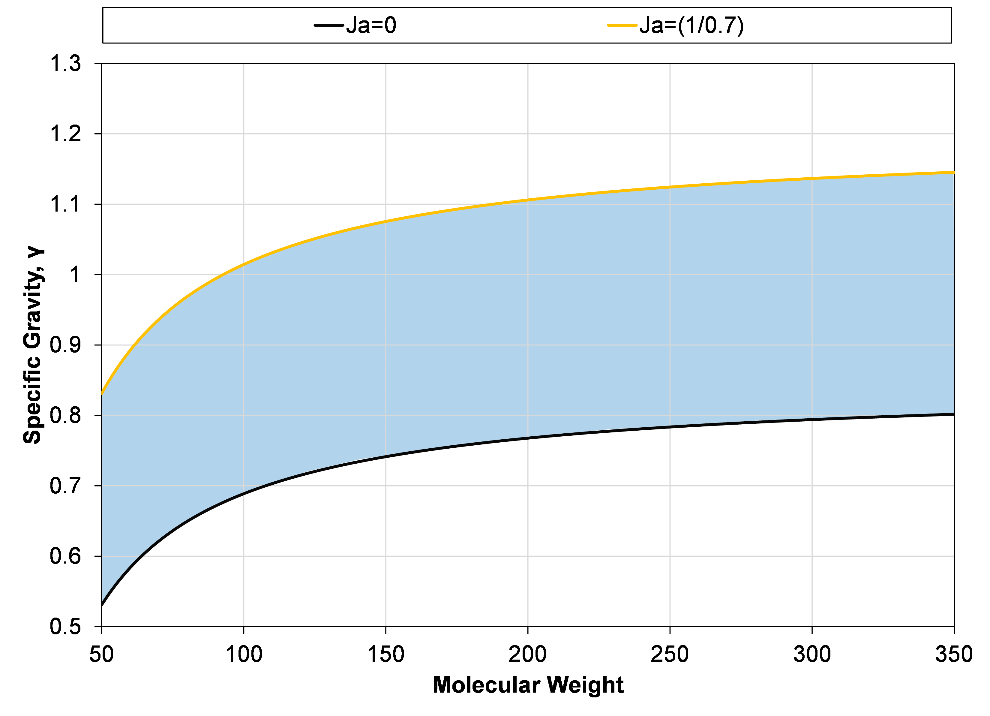paraffin_aromatic_bound_specific Figure 4: Specific gravity – molecular weight region (blue area) where single carbon number components can be when using the effective paraffin model with the choice deviation factor (δ) given in Equation \eqref{eq:delta_definition_with_jacoby}.

Twu Model

The Twu correlation for molecular weight is given by

$\begin{equation}\label{eq:twu_mw_definition} \ln⁡(M)=\ln [M_p (i)] \left(\frac{1+2f_p}{1-2f_p }\right)^2 \end{equation}$ $\begin{equation}\label{eq:fp_definition} f_p (M)=Δγ_M [x(M_p)+(0.193168 T_b^{-0.5} (M_p )-0.0175691)Δγ_M (M,M_p)] \end{equation}$ $\begin{equation}\label{eq:abs_x_definition} x(M_p)=|0.012342-0.328086 T_b^{-0.5} (M_p)| \end{equation}$ $\begin{equation}\label{eq:delta_gamm_m_definition} Δγ_M (M,M_p )=\exp[5(γ_p (M_p )-γ(M))]-1 \end{equation}$

and can be solved iteratively by estimating a molecular weight ($M$) then solving the left and right-hand side of Equation \eqref{eq:twu_mw_definition} separately and regressing on the molecular weight ($M$) until the left and right-hand sides are equal. The right-hand side is defined by the effective paraffin molecular weight $M_p(i)$ as defined in the previous section using Equations \eqref{eq:normal_paraffin_mw_correlation}, \eqref{eq:effective_paraffin_model}, and \eqref{eq:delta_definition_with_jacoby_with_specific_Ja}. The paraffin properties ($\gamma_p,T_b$) are calculated from Equations \eqref{eq:tb_twu_correlation}-\eqref{eq:alpha_definition} using the effective carbon number $(i)$ and not the normal paraffin carbon number $(I)$.

Excel Test File

We at whitson have made an Excel file with all the correlations above, that you can download for free here.