EOS Tuning

First time reading about EOS tuning?

Check out our article on the topic here!

The goal of the EOS Tuning feature is to fine-tune the initial C7+ characterized EOS model to match experimental PVT data. This data consists of the standard PVT experiments like the constant composition expansion (CCE), and more complex experiments like the slimtube experiment. The EOS Tuning feature does not consider the viscosity experiments, as this is covered in the Viscosity Modeling feature.

The EOS Tuning feature has four main inputs that you can adjust to impact your predictions. The inputs are:

• C7+ characterization case

• EOS parameter tuning

• Compositional adjustments

• Weight factors

All four of the inputs are covered in the sections below.

C7+ Characterization Case

You should always try to compare the different C₇₊ characterization cases you have saved! Unless you have distillation data which provides measured cut molecular weights, it can be hard to distinguish between the Twu and Effective Paraffin molecular weight models. The EOS tuning might shed some light on which model is most representative!

EOS Parameter Tuning

What would we recommend if this is your first time?

By default, only the BIPs are unlocked as regression in the tuning! If you don't get good results when running the EOS tuning case with just BIPs we recommend the following order of applying more tuning parameters:

1. Critical temperature (T_c) ramping.

2. Critical pressure (p_c) ramping.

3. Critical temperature heaviest fraction (T_c) CN+ multiplier.

4. Critical pressure heaviest fraction (p_c) CN+ multiplier.

5. Normal boiling point temperature (T_b) ramping.

6. Normal boiling point temperature heaviest fraction (T_b) CN+ multiplier.

EOS parameter tuning is a required step to develop an accurate model for petroleum mixtures with notable C₇₊ content because there are no truly predictive models that can estimate these parameters. The following C₇₊ component EOS parameters can be tuned in whitson^PVT:

• Critical temperature (T_c)

• Critical pressure (p_c)

• Normal boiling point temperature (T_b)

• Binary interaction parameters (dive deepk_ij) abbreviated as BIPs

The reason why the acentric factors are not on the list above is because they can be uniquely determined from the critical point and the normal boiling point which are both better-constrained physical properties. The BIPs between C₁ and the C₇₊ SCN components are adjusted using the Chueh-Prausnitz correlation. The default model parameters for the Chueh-Prausnitz correlation depend on which EOS model is used, and are as follows:

• Peng-Robinson 1979 (PR79): A=1 and B=1

• Soave-Redlich-Kwong (SRK): A=0 and B=1

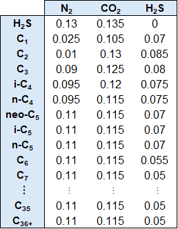
For the non-hydrocarbon and hydrocarbon BIPs, a set of default values are used as shown in the table below.

Table 1: BIPs for non-hydrocarbon and hydrocarbon pairs.

whitson^PVT offers several additional options, such as choosing an alternative first component for tuning (the default value is C₇), as well as letting you adjust the bounds by clicking the slider icon.

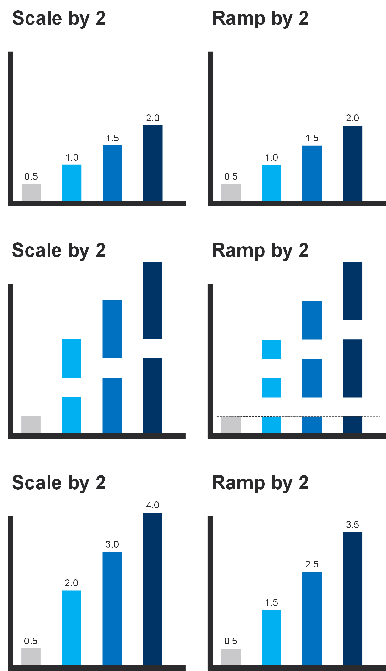
In whitson^PVT, two primary methods (ramping and scaling) are provided for adjusting the C₇₊ EOS parameter values, alongside an additional adjustment option for the heaviest fraction (the C₃₆₊ component). Both the ramping and scaling methods are detailed below.

Ramping is a single regression parameter tuning approach that aims to honor the growing uncertainty in the component properties for the heavier components. The method can be defined in Equation \eqref{eq:ramping_definition}.

$$\begin{equation}\label{eq:ramping_definition} \theta_x^* = \theta_{n-1} + R \cdot (\theta_x - \theta_{n-1}) \end{equation}$$

where \(\theta\) is the EOS property, the subscript \(n\) indicates the first plus component (usually set to 7), \(R\) is a scaling factor, and the subscript \(x\) indicates the C₇₊ component's SCN component name (i.e. \(x \geq n\)).

Scaling is a single regression parameter tuning approach that adjusts all component properties by a single scaling factor (\(S\)). The method can be defined in Equation \eqref{eq:scaling_definition}.

$$\begin{equation}\label{eq:scaling_definition} \theta_x^* = S \cdot \theta_x \end{equation}$$

where \(\theta\) is the EOS property and the subscript \(x\) indicates the C₇₊ component's SCN component name (i.e. \(x \geq n\)).

A comparison between ramping and scaling using a value of 2 for both \(R\) and \(S\) is given in the figure below

Figure 1: Comparison of scaling (left) and ramping (right) by a value of 2 starting from the second datapoint (light blue).

Compositional Adjustments

What would we recommend if this is your first time?

Before trying to apply the compositional adjustments, try some different cases without compositional regression! If you are applying the compositional adjustment, check if most or all the data goes in the same direction of better predictions.

Some datasets that we recomment checking when applying compositional adjustments are:

1. Saturation pressure.

2. CCE single-phase density.

3. MSS density, formation volume factor, and gas removed.

4. DLE density, oil formation volume factor, and gas removed.

5. Iduvidual experiment CVD liquid dropout.

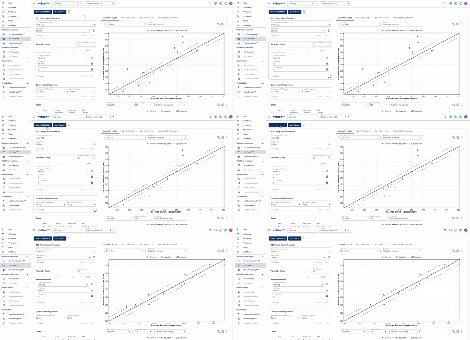
Compositional errors are real and can have a significant impact on your phase behavior predictions! However, with great power comes great resposibility. What do we mean by this? It is easy to match certain key predictions like saturation pressure, with very slight compositional adjustments, but this is not always the correct option! In general, we recommend changing the C7+ charaterization case (e.g. using Twu or Effective Paraffin MWs) and EOS tuning before adjusting the composition, if you plan to do so.

The two most common types of compositional errors that should be adjusted are:

• Recombination GOR

• Average molecular weight

Both of these options are adjustable in whitson^PVT! The recombination GOR adjustment allows you to tune the ratio of flashed gas to oil in the recombined fluid. For the compositional adjustment of the C₁ mole content, in whitson^PVT, the default constraint is 1 mole%. Round-robin studies have shown recombinations varying by up to 3 mole%. Modifying the average molecular weight of either the flashed oil or recombined fluid enables you to adjust the values used in the Gamma model. The choice of fluid is based on the availability of compositional data, with the priority being: (1) flashed oil, (2) separator oil, (3) recombined fluid.

The compositional adjustment is done induvidually for each sample in the EOS tuning.

Weight Factor Cases

What would we recommend if this is your first time?

This is an advanced feature, and unless you know what data you want to prioritize, we recommend that you stick to the default case!

Weight factor cases can be added to emphasize certain properties in the different PVT experiments. When making a custom weight factor case, you can choose a basis which automatically fills the property weights with the values of the basis case. This lets you make slight adjustments without needing to re-enter all the data.

EOS Tuning Results and Predictions

What would we recommend if this is your first time?

The top summary plots are there as a suggestion to help you check your model's tuning fit! We recommend going from top to bottom when comparing tuning cases!

Some other plots you might want to check:

• Multi-sample DLE data - In particular the oil formation volume factor and removed gas.

• Multi-sample MSS data - Same data as the DLE and the oil density.

• Induvidual sample CVD liquid dropout data.

• Induvidual sample CCE liquid dropout data.

The EOS tuning predictions are divided into four tabs on the right-hand side of the feature. Each tab's specific use is explained below.

The Summary Plots tab is composed of two plots, both showing multi-sample data predictions. There are three ways to display multi-sample data in whitson^PVT. The first is a cross-plot, which compares the lab reported data on the x-axis to the EOS predicted data on the y-axis. The second type is a by sample deviation plot, which shows the deviation for individual samples, defined by Equation \eqref{eq:deviation_definition}. The third type is a by property deviation plot, which lets you identify at what reported values your deviation starts to increase or decrease!

$$\begin{equation}\label{eq:deviation_definition} r = \frac{\theta_{calc} - \theta_{exp}}{\theta_{exp}} \cdot 100% \end{equation}$$

The first summary plot has a set of whitson recommended properties that we recommend you inspect and assess the quality of. The second (lower) summary plot is a by experiment plot for all samples containing data for that experiment type.

The second tab called PVT Experiments shows the experimental data and adjusted sample composition for individual samples. The top plot in this section lets you select a sample and its associated PVT experiment. You can then change the x- and y- properties freely. The second plot in this section shows the mole composition of this sample with compositional adjustments and characterized component molecular weights converting from mass to mole amounts. The adjusted composition is in the detailed EOS component slate!

The third tab is called EOS Properties and just like in the C7+ Characterization feature, this section shows you the EOS properties of the tuning case with a basis (x-axis) of either molecular weight, normal boiling point, or component name. This allows you to quickly check your tuned properties for thermodynamic consistency, either by looking for non-monotonic behavior or checking whether the data goes outside the pure compound properties (grey circles).

The fourth and last tab called Parameters Summary lets you compare the EOS tuning parameters for your different cases! This is a quick way to see how the tuning of your parameters is affected across different cases.

What's Next?

Having developed one or more EOS Tuning cases, the next step is to develop a viscosity model! You can read about how to do this here.

Do you have any questions or comments? Feel free to reach out to our support email: support.pvt@whitson.com.