Viscosity Modeling

First time reading about EOS tuning?

Check out our article on the topic here!

Once a tuned equation of state (EOS) model has been developed, the next step is to develop a model that can accurately predict viscosity. In whitson^PVT the Lohrenz-Bray-Clark (or LBC for short) is selected by default, but there are options for both the Pedersen and Pedersen for Eclipse. There are a multitude of other, more advanced models available in the literature, but there are several key reasons why the LBC model is prioritized here. First, it is the most commonly adopted model in most, if not all, commercial software which makes it possible to use across different software. Second, it is not too computationally costly like most other, more complex, models like the Pedersen pseudo-CSP model.

Orrick-Erbar Correction

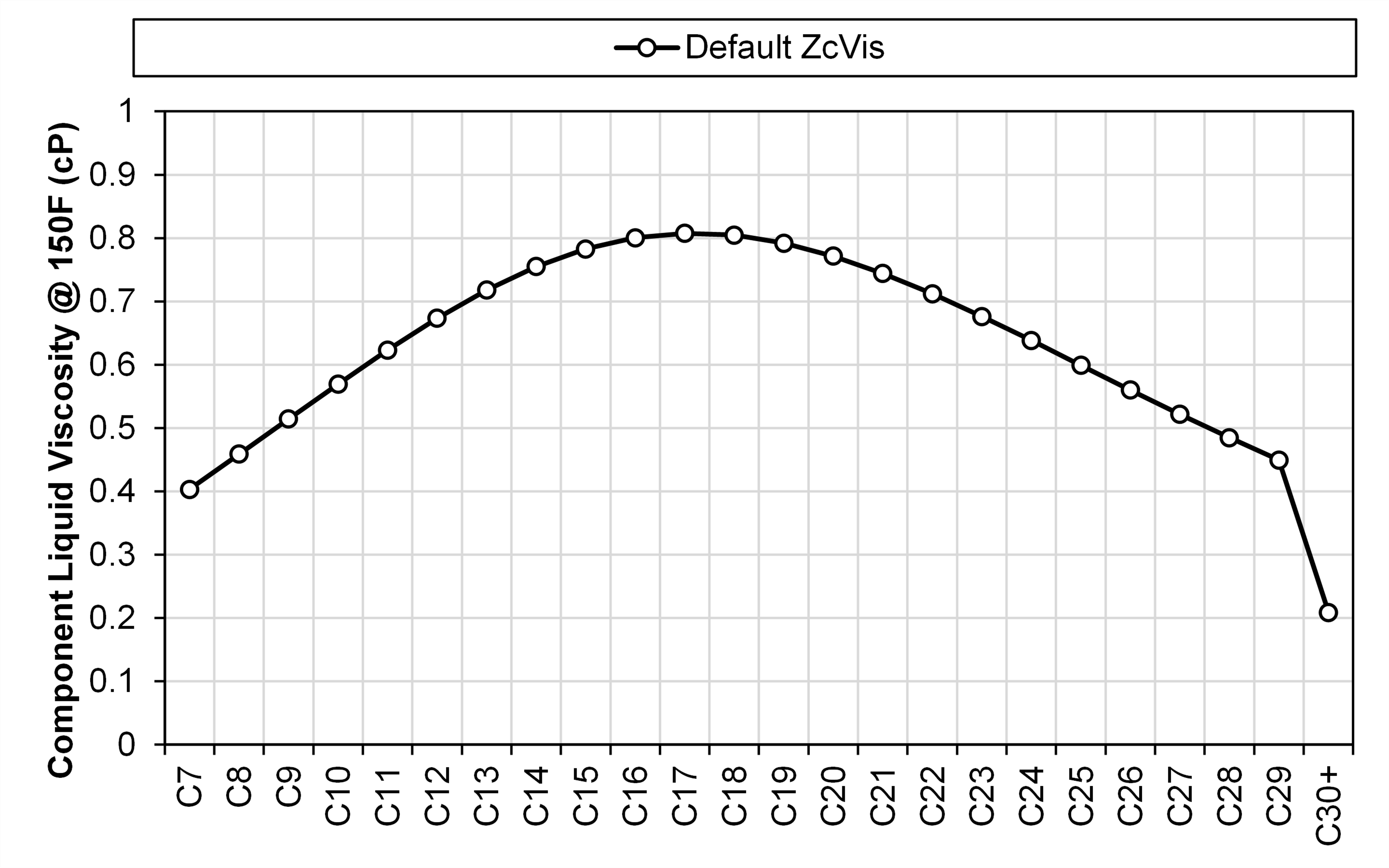
If you take any default PR or SRK EOS model and use the LBC viscosity model to predict the C7+ SCN component's liquid component viscosity, you might be supprised to see that they are going to behave non-monotonically. This results in your heaviest component (e.g. C₃₆₊) component viscosity being less than your C₇ SCN component viscosity. Not only is this non-physcial, but it will also have a significant negative impact on your mixture liquid viscosity predictions (even with a set of tuned LBC parameters). An example of this behavior is shown in Figure 1.

Figure 1: Example of non-monotonic behavior in C7+ SCN component liquid viscosity.

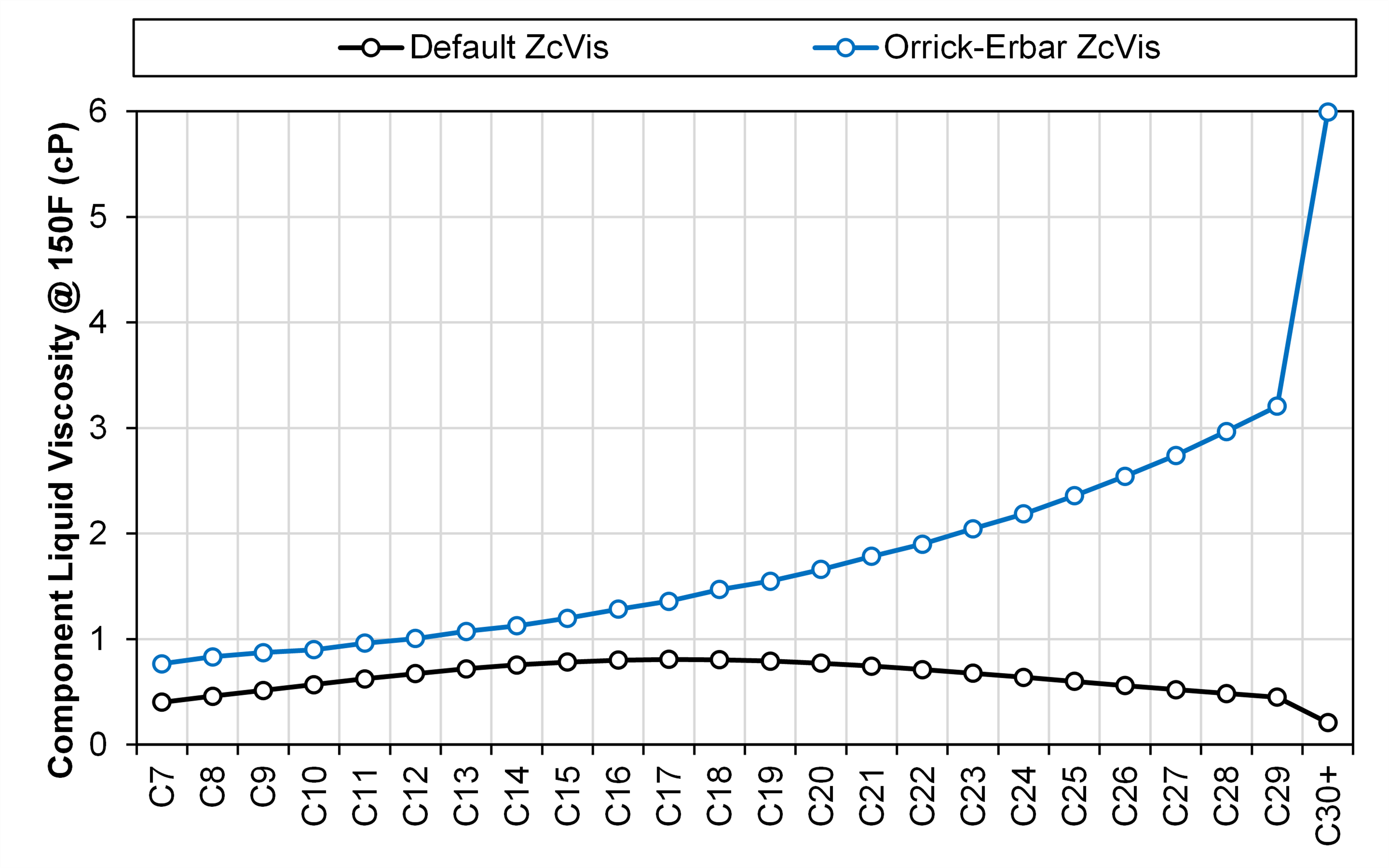
In whitson^PVT the Z_c,vis values are automatically adjusted to avoid this behavior. The initial liquid component viscosity values used to adjust the Z_c,vis values come from the Orrick-Erbar group contribution correlation. The resulting corrected component viscosities are shown in Figure 2.

Figure 2: Example of corrected C7+ SCN component liquid viscosity using the Orrick-Erbar correlation to adjust the ZcVis values.

Viscosity Model Basis

Similar to EOS Tuning, for viscosity modeling you must first specify the tuned EOS case! The EOS model you use will impact the viscosity predictions. In the same section as the viscosity model basis, you can also specify your weight factor case. This is a more advanced feature that should be used to fine-tune your results! If you are unsure what to use here, we recommend sticking to the default weight factors.

Parameter Tuning

What would we recommend if this is your first time?

By default, only the LBC P₄ parameter is unlocked. This parameter will impact the liquid-like viscosity predictions. In general, we recommend first trying to run this default case first to get a feel for how good the predictions are!

Our recommended progression of additional tuning parameters is as follows:

1. ZcVis ramping

2. Unlocking the P₃ parameter

3. Unlocking the P₂ parameter

Note that we do NOT recommend unlocking the P₁ or P₀ parameters unless (1) you are an experienced superuser and know what you're doing, or (2) you have a large set of gas viscosity data in your dataset.

For the viscosity model, there are two types of tuning parameters. The first is tuning of the Z_c,vis values. There are two methods for adjusting the C₇₊ SCN component Z_c,vis values: ramping and scaling. Both methods are explained in detail at the end of this section.

The second set of tuning parameters are the LBC polynomial coefficients. In general, the polynomial parameters have varying effects on different viscosity ranges. The most viscious fluids (liquids) are most heavily influenced by the P₄ paramter, while the least viscious are driven by the P₀ parameter. The P₄ parameter has the biggest impact on the most viscous fluids (liquids), while the P₀ parameter has the biggest impact on the least viscous fluids (gases). Since the LBC parameters are used in a 4th degree polynomial, it is possible for specific tuned coefficients to induce non-monotonic behavior, which should be avoided. In whitson^PVT it is simple to check this in the LBC Polynomial tab discussed in the Results and Predictions section below.

Ramping and scaling, the two main methods for adjusting C₇₊ component parameter values in whitson^PVT, are explained below.

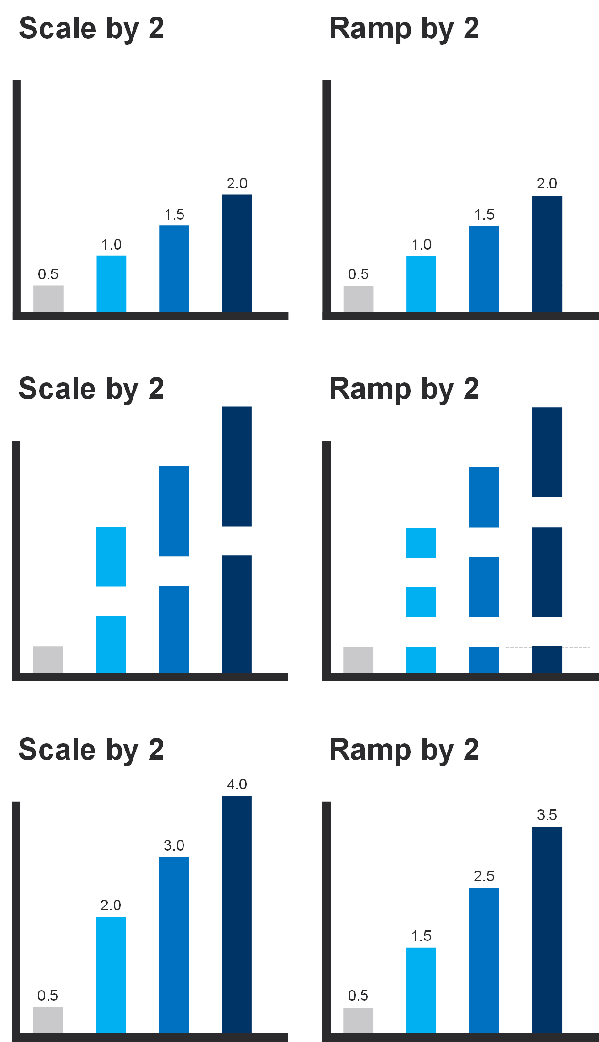
Ramping is a single regression parameter tuning approach that aims to honor the growing uncertainty in the component properties for the heavier components. The method can be defined in Equation \eqref{eq:ramping_definition}.

$$\begin{equation}\label{eq:ramping_definition} \theta_x^* = \theta_{n-1} + R \cdot (\theta_x - \theta_{n-1}) \end{equation}$$

where \(\theta\) is the component property, the subscript \(n\) indicates the first plus component (usually set to 7), \(R\) is a scaling factor and the subscript \(x\) indicates the C₇₊ component SCN component name (i.e. \(x \geq n\)).

Scaling is a single regression parameter tuning approach that simply sclaes all component properties up / down by a single scaling factor (\(S\)). The method can be defined in Equation \eqref{eq:scaling_definition}.

$$\begin{equation}\label{eq:scaling_definition} \theta_x^* = S \cdot \theta_x \end{equation}$$

where \(\theta\) is the component property, the subscript \(x\) indicates the C₇₊ component SCN component name (i.e. \(x \geq n\)).

A comparison between ramping and scaling with a value of 2 for \(R\) and \(S\) is given in the figure below

Figure 3: Comparison of scaling (left) and ramping (right) by a value of 2 starting from the second datapoint (light blue).

Viscosity Modeling Results and Predictions

The Viscosity Modeling predictions are divided into four tabs on the right-hand side of the feature. Each tab has a specific use and are explained below.

The Summary Plots tab is composed of one plot that shows both multi-sample data predictions. There are three ways to display multi-sample data in whitson^PVT. The first is a cross-plot that compares the lab reported data on the x-axis and the EOS predicted data on the y-axis. The second type is a by sample deviation plot, that shows the deviation defined by Equation \eqref{eq:deviation_definition} for individual samples. The third type is a by property deviation plot that lets you identify at what reported values your deviation starts to increase or decrease!

$$\begin{equation}\label{eq:deviation_definition} r = \frac{\theta_{calc} - \theta_{exp}}{\theta_{exp}} \cdot 100% \end{equation}$$

The summary plot shows the results for all samples that have viscosity experiment data. In this plot you can compare the predictions and the lab reported liquid and gas viscosity values.

The second tab called PVT Experiments shows the experimental data for individual samples. The plot in this section lets you select a sample and its assosiated viscosity experiment after which you can change the x- and y- properties freely.

The third tab is called LBC Polynomial and shows the LBC polynomial used to estimate the gas and liquid viscosity in the LBC model versus reduced density. The best way to read this plot is to think of the x-axis as how heavy your fluid is and the y-axis as your viscosity. In this way, you can see how the LBC parameter tuning impacts your gas (left side of the plot) and liquid (right side of the plot) viscosities relative to the default or other viscosity model cases.

The fourth and last tab called Parameters Summary lets you compare the EOS tuning parameters for your different cases! This is a quick way to see how your parameter tuning is affected for different cases.

What's Next?

Having developed one or more Viscosity Modeling cases, the next step is to store the detailed fluid model, and start developing your child models (i.e. your black-oil tables and lumped EOS models). You can read about how to do this here (for black-oil table generation) and here (for lumped EOS model generation).

Do you have any questions or comments? Feel free to reach out to our support email: support.pvt@whitson.com.