Specific Gravity Models

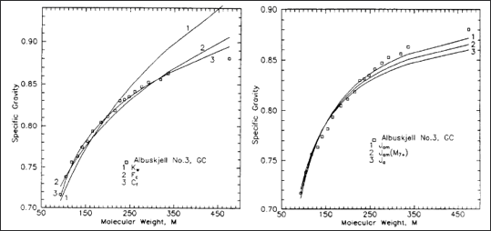
Figure 1: Relationship between specific gravity and molecular weight from a distillation experiment for the Norwegian field Albuskjell from Ingolf Søreide's PhD thesis. The lines are different correlations ranging from the Søreide model, Watson model, and Jacoby model.

Data like that provided by Søreide inhis PhD thesis (also shown in Figure 1) showns that specific gravity and molecular weight correlates, the question then becomes; what correlation we should fit to the data. There are a variety of different models that can be used, and a subset of the most common models will be covered here. Our recommendations for the choice of model will also be given together with the pros and cons of the different models.

Søreide Model

$$\begin{equation}\label{eq:soreide_model} \gamma(M) = \gamma_0 + C_f (M-M_0)^n \end{equation}$$

The Søreide model has four parameter values, (C_f, n, γ₀, M₀), and is given in Equation \eqref{eq:soreide_model}. The default values for the Søreide parameters are given by C_f=0.29, n=0.13, γ_{0=0.2855, and} M₀*=66. This is the only four parameter model and is general to the point of being able to predict all following correlations. The relationship between the Søreide model parameters and the other SG-model parameters will be given in the following sub-sections.

Watson Model

$$\begin{equation}\label{eq:watson_model} \gamma(M) = 6.0108 \cdot M^{0.17947} K_w^{-1.18241} \end{equation}$$

The Watson model has a single parameter (K_w) known as the Watson characterization factor. The Watson characterization factor is an indicator of the paraffinicity or aromaticity of the C₇₊ fraction. Values for K_w above 12-12.5 indicates that the fluid has mostly paraffinic component in it, while values around 10-11 indicate more aromatic components. Based on this, the initial value of the Watson characterization factor is set to K_w=12.

The relationship between the Equation \eqref{eq:watson_model} and Equation \eqref{eq:soreide_model} parameters is given below:

$$\begin{equation}\label{eq:soreide_to_watson} C_f = 6.0108 \cdot K_w^{-1.18241}; n=0.17947; \gamma_0 = 0; M_0 = 0 \end{equation}$$

Jacoby Model

$$\begin{equation}\label{eq:jacoby_model} \gamma(M) = 0.8468-\frac{15.8}{M}+J_a \cdot \left( 0.2456-\frac{1.77}{M} \right) = A + \frac{B}{M} \end{equation}$$

The original Jacoby model given in the first part of Equation \eqref{eq:jacoby_model} has a single parameter (J_a) known as the Jacoby characterization factor. The Jacoby characterization factor is an indicator of the paraffinicity or aromaticity of the C₇₊ fraction. Values for J_a ranges from 0 for paraffinic components to 1 for aromatic components. Based on this, the initial value of the Jacoby characterization factor is set to J_a=0.3.

The relationship between parameters in Equation \eqref{eq:jacoby_model} and Equation \eqref{eq:soreide_model} are given below

$$\begin{equation}\label{eq:soreide_to_jacoby} C_f = -15.8-1.77 \cdot J_a; n=-1; \gamma_0 = 0.8468+0.2456 \cdot J_a; M_0 = 0 \end{equation}$$

A generalized version of the Jacoby model is given in last part of Equation \eqref{eq:jacoby_model} that has two parameters (A,B). This is an empirical extrapolation based on the mathematic form of the Jacoby model given in the first part of Equation \eqref{eq:jacoby_model}. The relationship between the model parameters in the first and last part of Equation \eqref{eq:jacoby_model} is given below

$$\begin{equation}\label{eq:generalized_jacoby_to_jacoby} A = 0.8468+0.2456 \cdot J_a; B = -15.8-1.77 \cdot J_a \end{equation}$$

The relationship between the last part of Equation \eqref{eq:jacoby_model} and Equation \eqref{eq:soreide_model} are given below

$$\begin{equation}\label{eq:soreide_to_generalized_jacoby} C_f = B; n=-1; \gamma_0 = A; M_0 = 0 \end{equation}$$

Molar-Volume Model

$$\begin{equation}\label{eq:molar_volume_model} \gamma(M) = \frac{M}{a \cdot M + b} \end{equation}$$

The molar volume correlation has two parameters (a,b) that will also be referenced to as the slope (a) and intercept (b) as these are they are the slope and intercept of the straight line that results from plotting γ/M versus M. The default values for the molar-volume model are a=1 and b=40.412.

The relationship between parameters in Equation \eqref{eq:molar_volume_model} and Equation \eqref{eq:soreide_model} are given below

$$\begin{equation}\label{eq:soreide_to_molar_volume} C_f = \frac{-b}{a^2}; n=-1; \gamma_0 = \frac{1}{a}; M_0 = -\frac{b}{a} \end{equation}$$

Some motivation for the molar-volume correlation is found when plotting molar volume (M / γ) versus molecular weight (M) for the normal paraffins. This is shown in Figure 2, and from the R² it is clear that the straight-line fit is a good approximation. Re-arranging the linear equation to solve for specific gravity yields Equation \eqref{eq:molar_volume_model}.

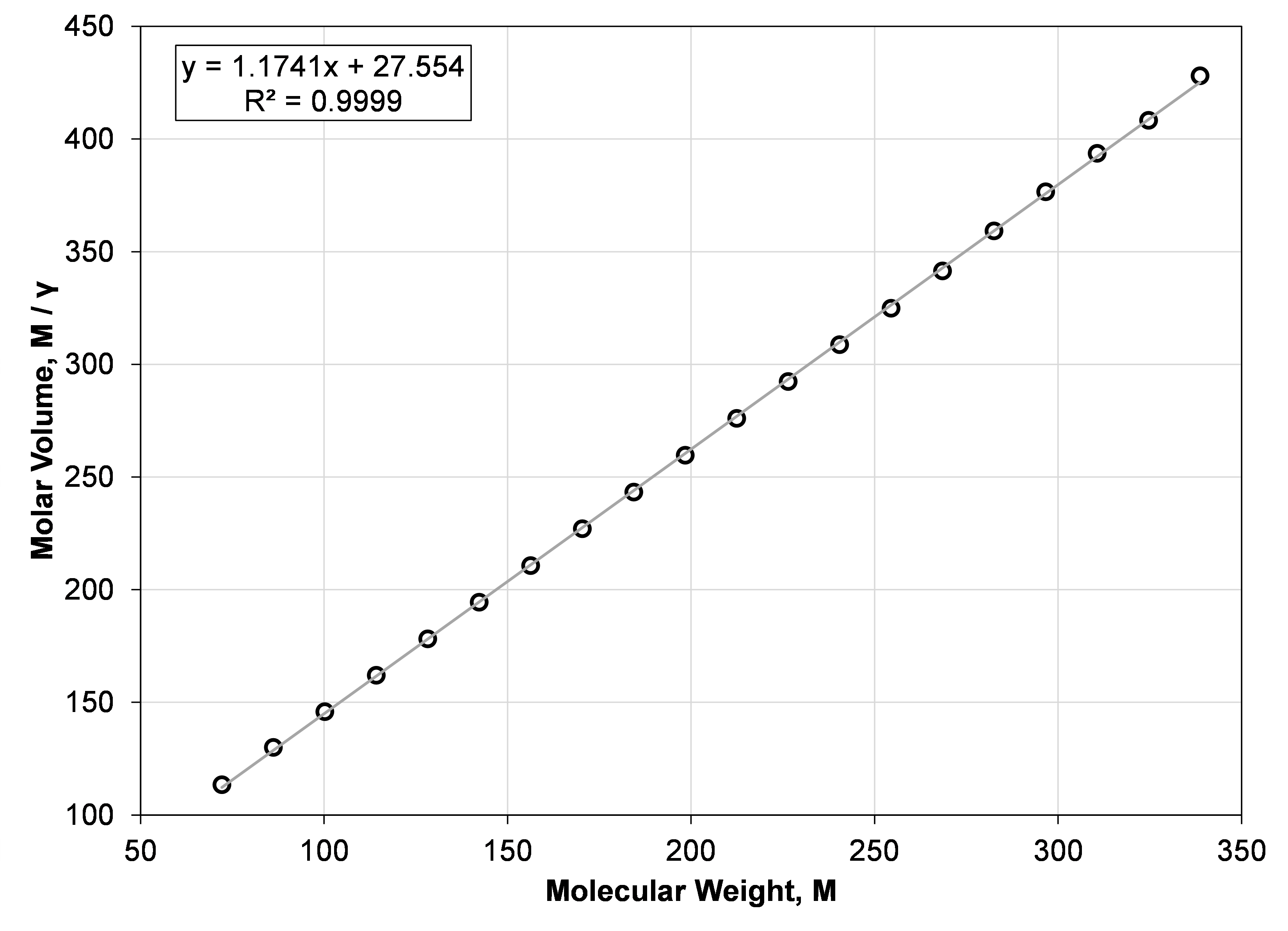
Figure 2: Straight-line fit of the normal paraffin molecular weight and molar volume from n-C₅ to n-C₂₄.

Pedersen Model

$$\begin{equation}\label{eq:pedersen_model} \gamma(M) = A + B \cdot \ln(I); I : M_p = M_{CH2} \cdot I + M_{H2} \end{equation}$$

where M_CH2 = 14.0269, and M_H2 = 2.01588.

The Pedersen model has two parameters (A,B) and uses the single carbon number (I) as an input as shown in Equation \eqref{eq:pedersen_model}. To convert from molecular weight to the effective single carbon number, simply re-arrange Equation \eqref{eq:pedersen_model} to solve for I instead of M. The Pedersen model cannot be analytically related to the Søreide model but can be curve fit by regression or analytically solving for the Søreide parameters assuming four points from the Pedersen model.

Excel Test File

We at whitson have made an Excel file with all the correlations above, that you can download for free here.