Volve Field Case Study
The Volve field makes for a great case study, since it has a lot of different data. The Volve dataset ranges from standard PVT experiments, to more advanced gas EOR experiments, and even detailed distillation data. The dataset has both oil-based mud (OBM) contaminated, and clean sample composition data.
The only downside of the dataset from the Volve field is that there is not a lot of variation in the fluid type (think GOR range). It is basically the same black-oil type data for most of the data, with the exception of the swelltest data.
Compositional & PVT Data
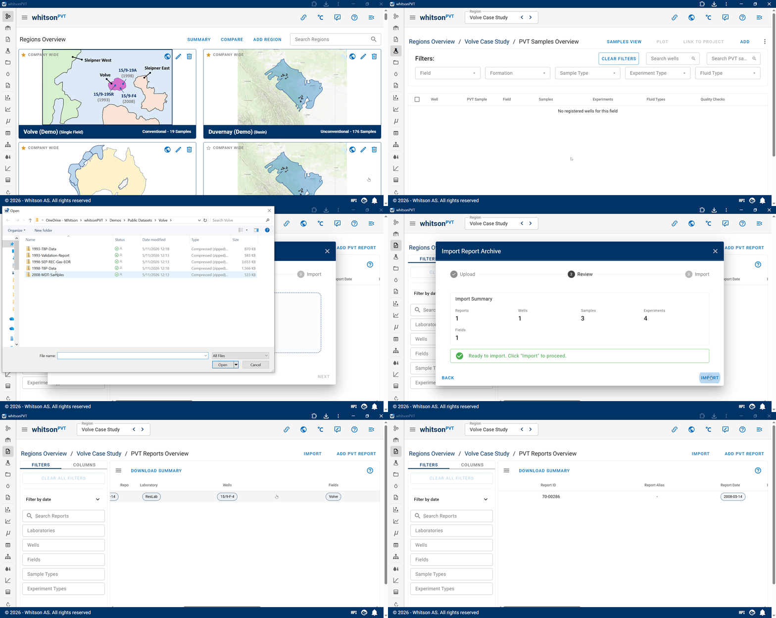
Utilizing the whitsonPVT automatic data import feature, we can seemlessly add PVT reports to your domain, without the need for manual data digitalization! You can find the relevant data that we will look at in this case study below.
-
2008 MDT Samples - Report here
- Two OBM contaminated MDT samples with extended (C36+) compositions.
- Both samples have constant composition expansion (CCE) experiment.
- One sample has multi-stage separator (MSS) experiment.
-
1998 Separator Recombined Sample - Report here
- Separator recombined sample with missing separator oil data.
- CCE and gas EOR experiements.
-
1993 & 1998 Crude Oil Samples - Report here and here
- Extended true boiling point (TBP) distillation experiment for both crude oil samples.
You can easily upload the reports in your private Region by following the steps shown in the video below.
Fluid Model Development
The fluid model development in this case study will have a bit more "educational" format than the other studies, and this is because we want to showcase the different types of data and functionality in this case. The other case studies are meant to give a more "industrial" application flavor.
Single-Sample Model Development
It has been more or less industry standard that developing fluid models is done on few or even a single sample. This is not something that we recommend (if it can be avoided), and we will attempt to showcase this in this case study.
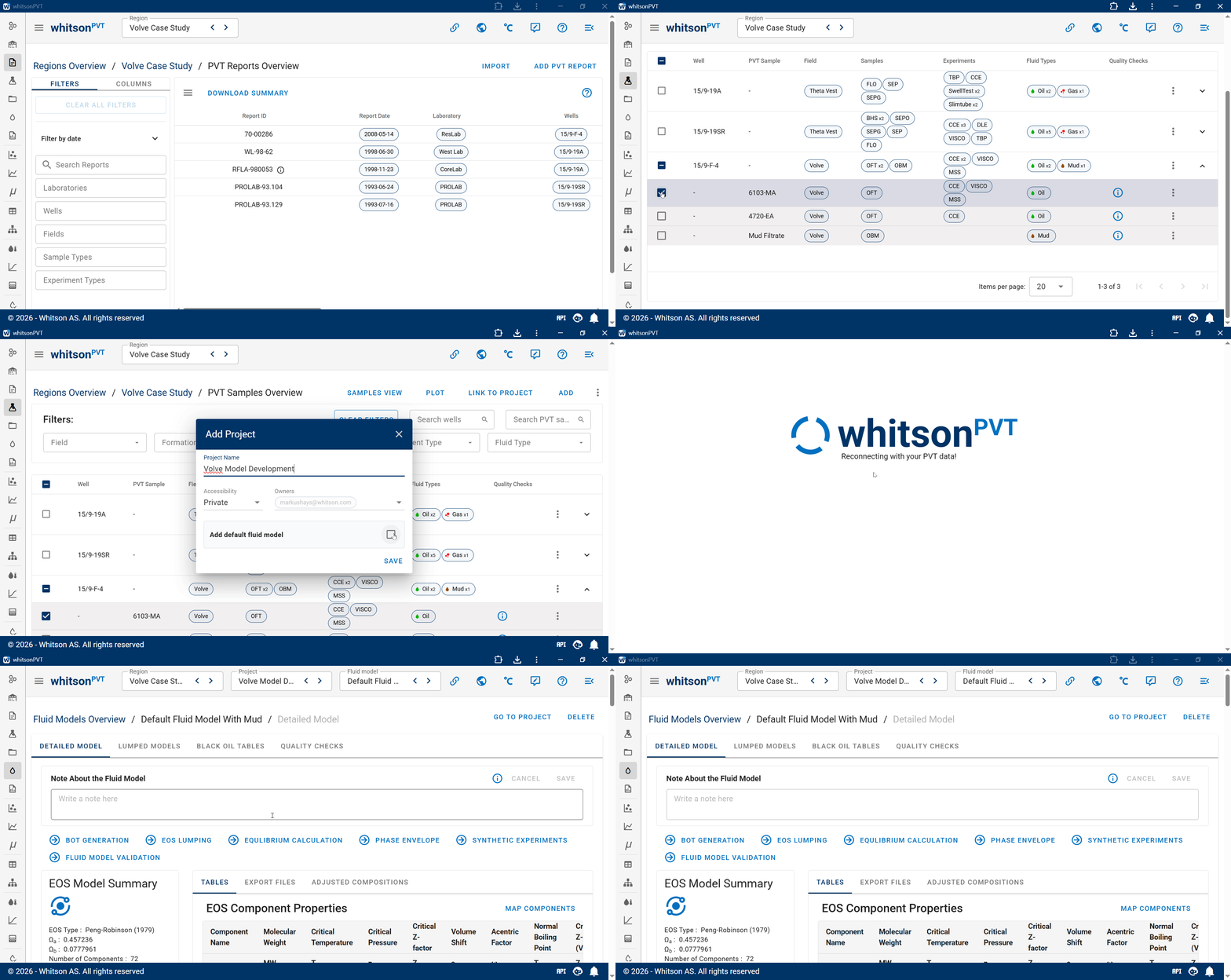
To perform the single-sample model development, we will select the sample named 6103-MA from the well named 15/9-F-4, and add it to a project that we will call Volve Model Development. You can see how this is done below.
Before we start with the fluid model development, I want to first test and see the predictions using a default EOS (with no tuning). You can see the predictions of the PVT data in the Fluid Model Validation feature, as shown below.
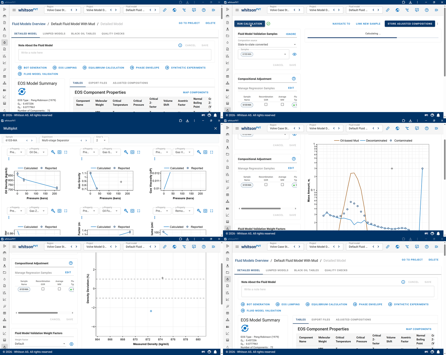
You can see that the predictions of the PVT experimental data does quite well, although the flashed oil density is about 2% underpredicted (which is more than we would like). Now let's see if we can do any better!
Going back to the project overview page, we are now going to start the fluid model development. The first step is the fluid model development is C7+ characterization, where we will get a look at the following topics:
-
Initial EOS model parameters
-
OBM contamination splitting (decontamination)
-
Gamma molar distribution model
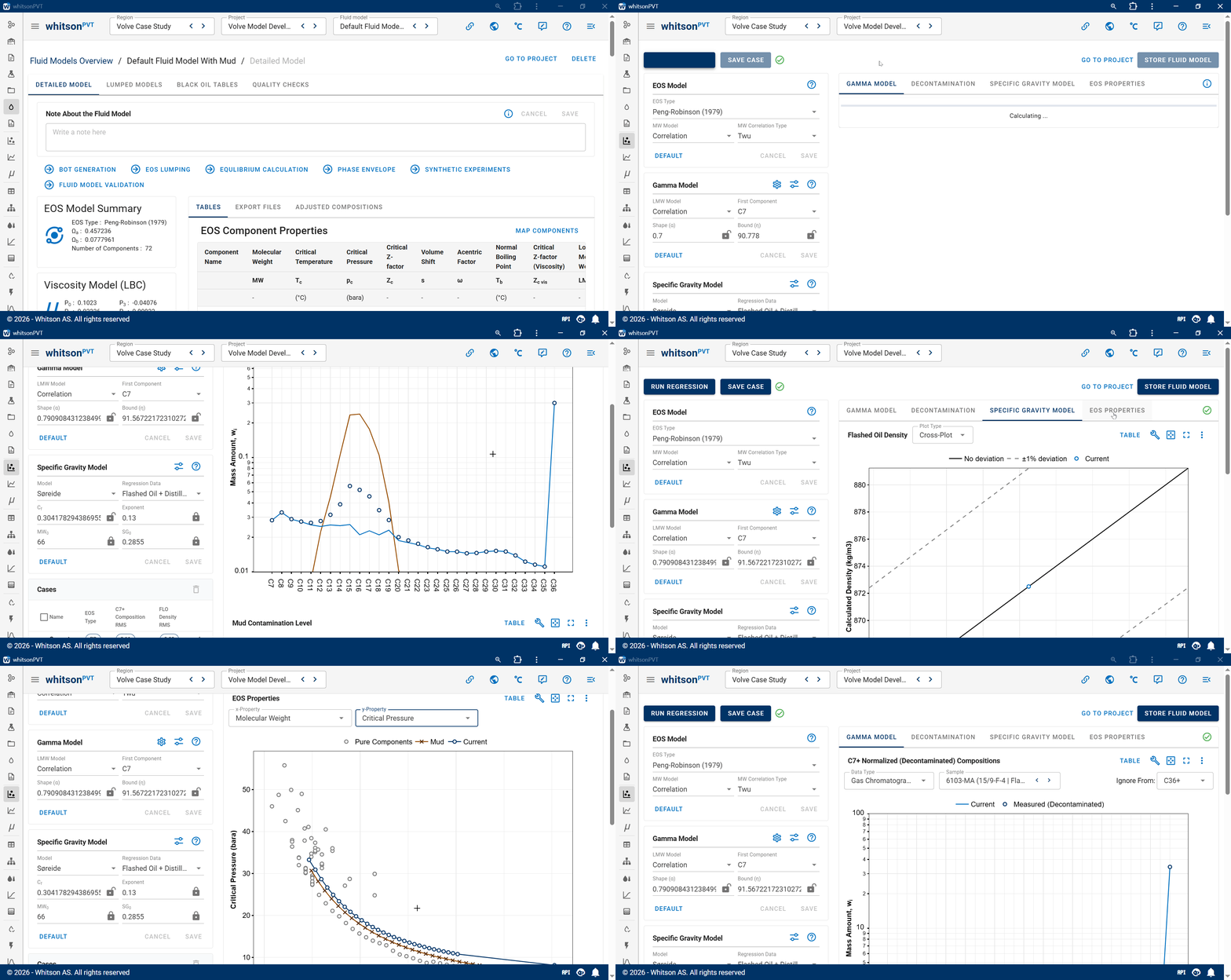
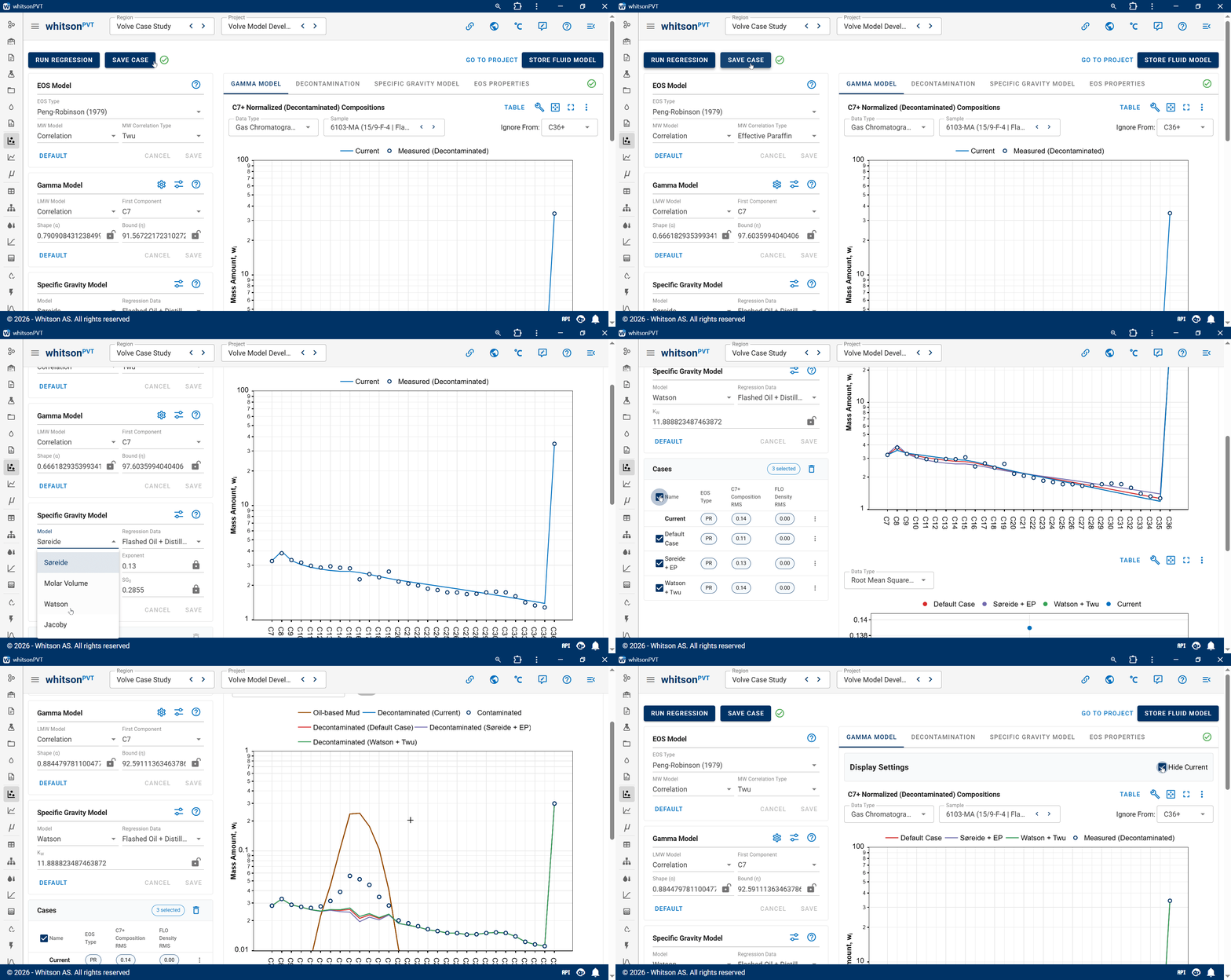
One of the main issues with single-sample modeling is that the fluid model development becomes a highly underspecified regression problem, meaning that there are a lot of solution that yield an equally good result. We can highlight this in whitsonPVT by saving and displaying multiple cases. You can see several cases being run, saved, and compared below.
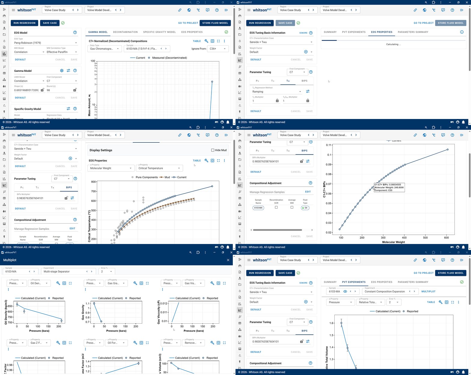
Moving on to the EOS tuning, you can pick you favorite C7+ characterization case as the starting point, and run the whitsonPVT default EOS tuning. By default, it is only the binary interaction parameters (BIPs) between C1 and the C7+ components (C7, C8, C9, etc. until C36+). The BIPs are initially estimated using the Cheuh-Prausnitz correlation, and are modified by a single scaling factor for all C1-C7+ BIPs. This approach was shown by Katz and Firoozabadi to have a significant impact on the phase behavior predictions. You can learn more about BIPs tuning here.
In the example below, you can see the predictions for the EOS model tuning in this case using the whitsonPVT default C7+ characterization.
Finally, we can run the viscosity modeling. We typically recommend starting your viscosity modeling byt trying to use the Lohrenz-Bray-Clark (LBC) viscosity model, for the simple reason that it is a simple and robust model that you can be pretty sure is implemented in any commercial software. Other methods exists, like the Pedersen model (sometimes called the CSP model) or various friction theory models, but thes are typically more computationally expensive to run, and are not necessarily implemented in all relevant simulation software that you would need your fluid model to be used in.
For this case, we will stick to the LBC model, but in addition to tuning the LBC polynomial coefficient P4, we will also scale the C7+ Orrick-Erbar corrected Zc,vis values by a single scaling factor. You can see how this is done below.
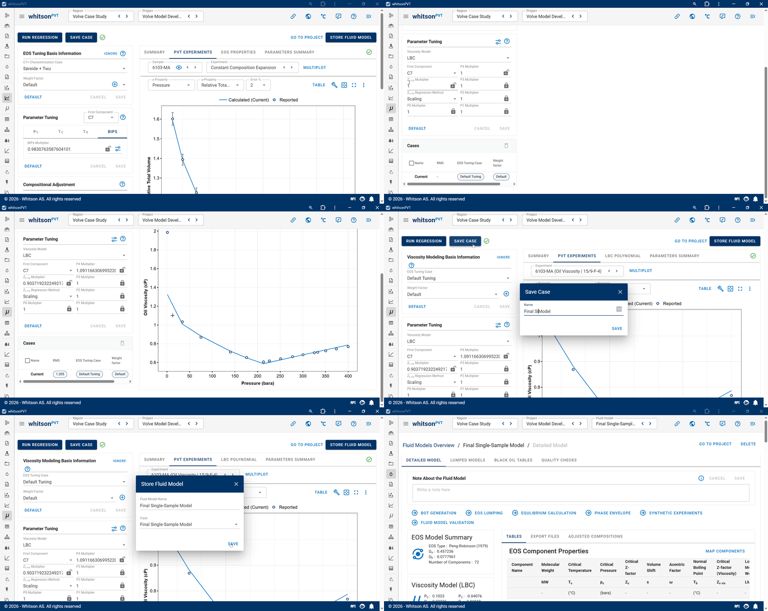
We finalized the fluid model development by clicking the STORE FLUID MODEL button, which takes our work-in-progress fluid model and locks it in and stores it in the Fluid Models overview page.
C7+ Compositional Distribution - Real or Fake?
If you're following along in whitsonPVT, you might have noticed something interesting in the decontaminated flashed oil mass composition. In whitsonPVT we use the physically consistent subtraction method when estimating the contamination level. Unlike other methods, like skimming, where you assume a smooth straigh line behavior, this can result in compositions that "wiggle" around. The question I pose to you is: Is this real, an artifact of the decontamination, or a measurement error (or something else)?
How can we test this? We can test it by finding another independent sample that we know is not OBM contaminated and compare the C7+ mass distribution. Luckily, we have another C36+ extended sample from another report for the separator recombined sample. Since the sample is taken at the separator, there is not going to be any impact from the mud. The sample is also from an entirely different report and was taken 10 years prior to the contaminated MDT oil sample.
You can see how we can add this sample to the project we're working on, to see the predicted composition and how the separator sample C7+ mass distribution compared to the whitsonPVT decontaminated MDT sample C7+ mass distribution.
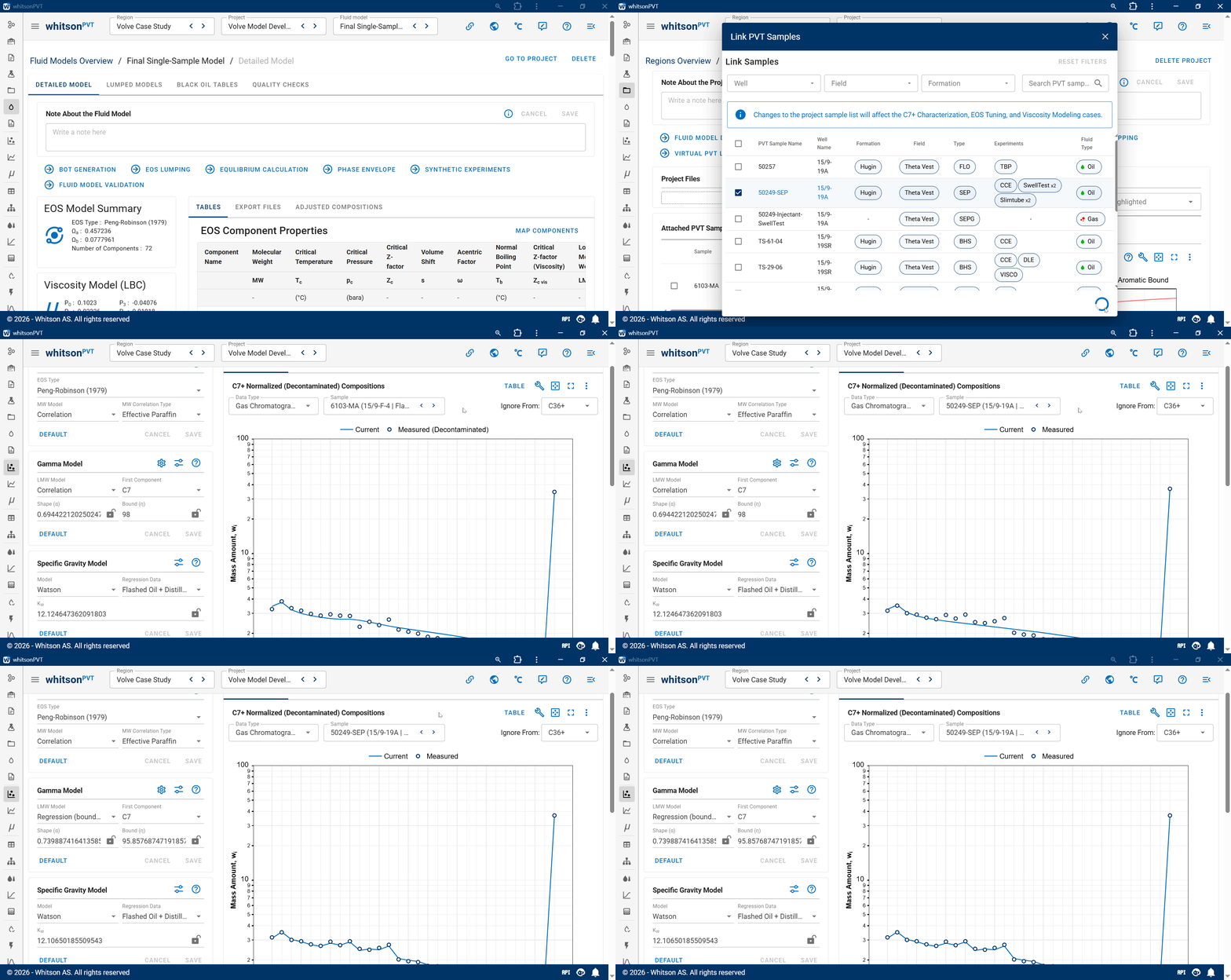
You can also see that applying the LMW Regression yields a much better prediction of the mass composition data. The sample mass composition distribution seem to be very similar, which is an indication that the "wiggle" that we see for the decontaminated MDT sample is real, and not an artifact that we should "smooth away" like the skimming method would!
Adding Distillation Data
With only a single flashed oil density, we don't really have enough data to create a specific gravity relationship that represents the fluid character. You might ask why we would care about the "specific gravity relationship", and a partial answer to this is that the component critical properties initial estimates are dependent on the estimated component specific gravities. You can read more about this here. The component specific gravity is also used to determine the component volume shifts, that you can learn more about here.
There are different ways of creating a more representative component specific gravity relationship. The first is to have reservoir samples with a broader GOR range (gas and oil samples for example). However, this is not always the case like for the Volve field.
The best way to get a component specific gravity relationship is to have true boiling point (TBP) distillation data, where the distillation cut specific gravities are measured. For Volve, there are two such dataset. These datasets are particularly useful since they have extended analysis beyond what is normal. Both measured specific gravities and molecular weights are measured for each distillation cut! This is really useful for the C7+ characterization. You can see the impact of adding this data type below.
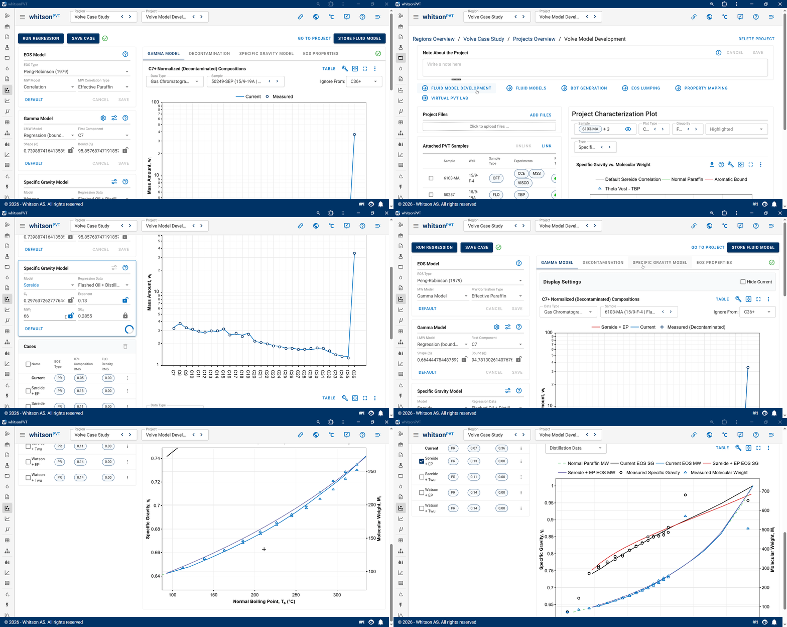
You can see that adding the distillation data gives a much better component specific gravity and molecular weight description than the initial estimate that we developed without access to the distillation data.
By constraining the specific gravity and molecular weight models, we are limiting the possible initial estimated for the EOS properties! This will limit the amount of EOS tuning that is required to develop accurate EOS model.
EOS Tuning
Using the final C7+ characterization case that was developed using the MDT sample, the separator recombined sample, and the distillation data, we can now continue on with the EOS tuning.