Fluid Compressibility - It's not measured, it's calculated!

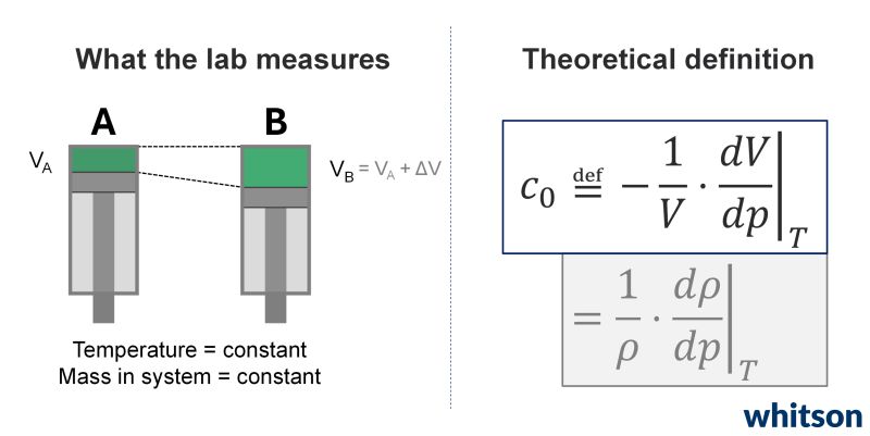
This post series explains why fluid compressibility is often misunderstood in PVT and reservoir engineering workflows. The central point is that compressibility is not directly measured in the lab. It is calculated from measured pressure-volume data, and that calculation depends on estimating a derivative.

For a single-phase, isothermal, closed fluid system, compressibility is based on the pressure derivative of volume:

$$c = -\frac{1}{V}\left(\frac{dV}{dp}\right)_T$$

That derivative is the source of much of the difficulty. Small differences in how pressure-volume data are fitted, smoothed, rounded, or differenced can lead to much larger differences in the calculated compressibility. Across the series, the posts move from definition and intuition to numerical methods, curve fitting choices, finite difference accuracy, pressure step size, and significant-digit sensitivity.

The overall conclusion is that matching or comparing "lab compressibility" values requires care. The reported compressibility is itself a derived quantity, not a direct measurement, and different calculation methods can produce meaningfully different results from nearly identical volume data.

Post-by-Post Summary

Post 1: Definition and Motivation

The series begins by questioning common claims about fluid compressibility, including the idea that equation-of-state models are poor when they do not match lab-reported compressibility. Before evaluating such claims, the post establishes the definition of single-phase isothermal fluid compressibility.

Key ideas:

• Compressibility is defined for a constant-temperature, closed, single-phase fluid system.
• The expression depends on volume, pressure, and the derivative of volume with respect to pressure.
• Derivatives are not directly measured in standard lab work, which means compressibility must be calculated from measured data.
• This distinction between measured quantities and derived quantities sets up the rest of the series.

Source: Post 1

Post 2: Pressure-Volume Intuition

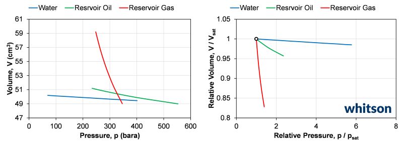
The second post builds intuition by comparing pressure-volume behavior for reservoir gas, reservoir oil, and reservoir water. Water requires only a small volume change to produce a large pressure change, gas requires a much larger volume change for the same pressure change, and oil lies between the two.

The finite-change intuition is:

$$\frac{\Delta V}{\Delta p} \approx \frac{dV}{dp}$$

Key ideas:

• Different fluids have very different pressure-volume relationships.
• The ratio dV/dp, or its finite change approximation delta V / delta p, helps quantify the relationship.
• Taking the limit of delta V / delta p leads to the derivative used in the compressibility expression.
• The derivative is the mathematical bridge between measured pressure-volume data and calculated compressibility.

Source: Post 2

Post 3: Visualizing the Derivative from Real Data

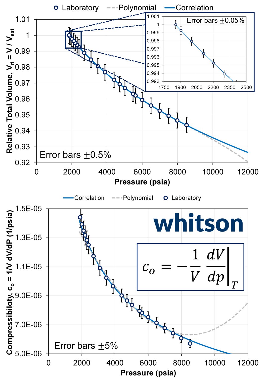
The third post uses measured relative total volumes from a real petroleum reservoir gas system:

$$V_{rt} = \frac{V}{V_{p_{sat}}}$$

A curve-fitting tool is used to fit an equation to the data, after which the analytical derivative of that fitted curve can be calculated and visualized at specific pressures.

Key ideas:

• Real lab pressure-volume data can be fitted with a smooth mathematical model.
• Once a model is fitted, its analytical derivative can be calculated.
• The fitted-model derivative can be treated as a reference case for comparing numerical derivative approximations.
• This sets up the later comparison between analytical derivatives and finite difference methods.

Source: Post 3

Post 4: Derivative Approximation Methods

The fourth post introduces several ways to approximate the derivative needed for compressibility. The post compares a pressure-volume curve, an analytical reference derivative, and numerical approximations.

Methods introduced:

• Forward finite difference: uses the current point and the next pressure point.

$$\left.\frac{dV}{dp}\right|_{p_k} \approx \frac{V_{k+1} - V_k}{p_{k+1} - p_k}$$

• Backward finite difference: uses the current point and the previous pressure point.

$$\left.\frac{dV}{dp}\right|_{p_k} \approx \frac{V_k - V_{k-1}}{p_k - p_{k-1}}$$

• Local quadratic polynomial: uses the current point, previous point, and next point, then differentiates the fitted local polynomial.

Key ideas:

• Numerical derivative method choice matters.
• Different derivative approximations can produce visibly different results.
• Lab-reported compressibility values are calculated from data, so the calculation method behind them matters.

Source: Post 4

Post 5: Curve Fit Choice Can Change Compressibility

The fifth post compares two equations fitted to lab-measured volume data: a cubic polynomial and a log-normal cumulative distribution function. Both fit the volume data extremely well, with less than about 0.02 percent deviation per data point, but they produce dramatically different compressibility estimates.

The important relationship is that the curve fit is not the final target; the derivative of the curve fit is what enters compressibility:

$$c(p) = -\frac{1}{V(p)}\frac{dV(p)}{dp}$$

Key ideas:

• A very good fit to pressure-volume data does not guarantee a good compressibility estimate.
• Compressibility depends on the derivative of the fit, not only the fit itself.
• The cubic polynomial, although commonly used in some lab workflows, performed poorly for this example.
• The "correct" compressibility estimate is not obvious because the derivative is inferred, not measured.

Source: Post 5

Post 6: Forward and Backward Finite Difference Accuracy

The sixth post focuses on forward and backward finite difference methods. A fitted base-truth model is used as a reference, and the finite difference slopes are compared against its analytical derivative.

The finite difference slope is converted to compressibility at a pressure point as:

$$c_k \approx -\frac{1}{V_k}\left(\frac{\Delta V}{\Delta p}\right)_k$$

Key ideas:

• Forward and backward finite differences use only two points at a time.
• Their error depends strongly on pressure step size.
• As the pressure step delta p decreases, the approximation error decreases.
• Large lab pressure steps can therefore create material error in calculated compressibility.

Source: Post 6

Post 7: Local Quadratic Polynomial Approximation

The seventh post presents an alternative derivative estimate using a local quadratic polynomial. This method fits a local polynomial through the current pressure-volume point and its two neighboring points, then calculates the analytical derivative of that local polynomial at the current point.

For a local quadratic fit:

$$V(p) \approx ap^2 + bp + c$$

the local derivative is:

$$\frac{dV}{dp} \approx 2ap + b$$

Key ideas:

• Using both neighboring points gives a better local slope estimate than simple forward or backward finite differences.
• The local quadratic method more closely follows the base-truth analytical derivative in the example.
• Even this method is still an approximation; "perfect" is not a well-defined target when the underlying derivative is not directly measured.

Source: Post 7

Post 8: Sensitivity of Compressibility to Derivative Calculation

The eighth post quantifies how sensitive compressibility can be to the derivative calculation. A cubic polynomial and a log-normal CDF both match the measured volume data very closely, with less than about 0.05 percent deviation at each pressure. However, their calculated compressibility values can diverge much more, especially near saturation pressure.

Key ideas:

• Tiny differences in volume matching can become much larger differences in compressibility.
• In the example, roughly 0.01 percent deviation in pressure-volume data can scale to roughly 10 percent deviation in calculated compressibility near saturation pressure.
• This represents an amplification of about three orders of magnitude.
• Extrapolation beyond the lab pressure range can make fitted equations diverge rapidly.

Source: Post 8

Post 9: Finite Difference Method, Step Size, and Precision

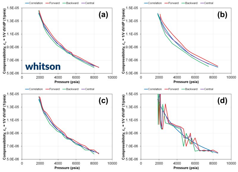
The ninth post compares forward, backward, and central difference methods under different data conditions. It examines full precision, reduced pressure steps, and reduced significant digits.

The central difference estimate is:

$$\left.\frac{dV}{dp}\right|_{p_k} \approx \frac{V_{k+1} - V_{k-1}}{p_{k+1} - p_{k-1}}$$

Key ideas:

• Central difference most closely matched the base-truth model when full precision and all pressure steps were used.
• Forward and backward methods were more sensitive to pressure step size.
• Reducing the number of pressure steps worsened finite difference performance.
• Reducing significant digits caused large errors, especially when only three significant digits were retained.
• Data resolution and rounding can be as important as the derivative method itself.

Source: Post 9

Method Comparison

Method	Data Used	Main Advantage	Main Risk
Cubic polynomial global fit	All measured volume data	Simple, common, smooth analytical derivative	Can fit volumes well but give poor derivative behavior
Log-normal CDF global fit	All measured volume data	Smooth fit with better behavior in the shown example	Still model-dependent and sensitive outside the data range
Forward finite difference	Current point and next point	Simple and easy to compute	Sensitive to pressure step size and one-sided bias
Backward finite difference	Current point and previous point	Simple and easy to compute	Sensitive to pressure step size and one-sided bias
Central difference	Points on both sides of current point	Better approximation in the shown comparison	Requires neighboring data on both sides
Local quadratic polynomial	Current, previous, and next points	Gives a better local derivative estimate than simple one-sided differences	Still sensitive to spacing, noise, and data precision

Main Takeaways

• Compressibility is calculated from pressure-volume data; it is not measured directly.
• The derivative dV/dp is the core difficulty in compressibility estimation.
• A curve can match measured volumes very well while giving poor derivative behavior.
• Numerical derivative estimates depend on method, pressure spacing, and data precision.
• Central or local polynomial methods generally performed better than one-sided finite differences in the examples shown.
• Rounding and reduced significant digits can severely degrade finite difference estimates.
• Near saturation pressure, small volume-fit differences can be amplified into much larger compressibility differences.
• Claims about matching lab compressibility should consider how the lab value was calculated.

Practical Implications

When comparing an equation-of-state model or other PVT model against lab-reported compressibility, it is not enough to ask whether the model matches the reported values. A more useful comparison asks:

• Which pressure-volume data were measured?
• What pressure spacing was used?
• How many significant digits were retained?
• Was the derivative calculated using finite differences, a curve fit, smoothing, or another method?
• Was the fit evaluated inside or outside the measured pressure range?
• How sensitive is the reported compressibility to the chosen derivative method?

The series makes a strong case that compressibility matching is partly a physics problem, partly a numerical differentiation problem, and partly a data-processing problem.